智能信息处理综合实践

7.1-7.3 风险评估模型效果评价方法 & ROC & AUC

widcardw

SPA

7.1 风险评估模型效果评价方法

准确性
- ROC 曲线 (receiver operating characteristic curve)
  - 通过 真正率 TPR 和 假正率 FPR 两个指标进行绘制
    - 真正率表示模型 推测为真，而 实际也为真 的概率
    - 假正率表示模型 推测为真，但 实际为假 的概率
  - 曲线与横轴之间的面积称为 AUC (area under of curve)
    - AUC 的取值范围一般在 $[0.5,1]$ ，值越大表示模型效果越好
- KS 检验
稳定性：模型是在特定时间点开发的，是否对外部样本有效 需要经过 稳定性测试。群体稳定性指标 (PSI) 是最常用的模型稳定性评价指标
可解释性：在逻辑回归和随机森林模型中，考量各个解释变量对目标变量预测结果的影响程度，可以得到模型指标重要性

智能信息处理综合实践

7.1-7.3 风险评估模型效果评价方法 & ROC & AUC

widcardw

SPA

7.1 风险评估模型效果评价方法

准确性
- ROC 曲线 (receiver operating characteristic curve)
  - 通过 真正率 TPR 和 假正率 FPR 两个指标进行绘制
    - 真正率表示模型 推测为真，而 实际也为真 的概率
    - 假正率表示模型 推测为真，但 实际为假 的概率
  - 曲线与横轴之间的面积称为 AUC (area under of curve)
    - AUC 的取值范围一般在 $[0.5,1]$ ，值越大表示模型效果越好
- KS 检验
稳定性：模型是在特定时间点开发的，是否对外部样本有效 需要经过 稳定性测试。群体稳定性指标 (PSI) 是最常用的模型稳定性评价指标
可解释性：在逻辑回归和随机森林模型中，考量各个解释变量对目标变量预测结果的影响程度，可以得到模型指标重要性

了解 TPR & FPR

以糖尿病为例，糖尿病的重要诊断方法为随机静脉血浆葡萄糖含量 $\geqslant 11.1 \mathrm{mmol/L}$

了解 TPR & FPR

	样本 1	样本 2	合计
诊断试验 1	43 真阳 TP	5 假阳 FP	48
诊断试验 2	7 假阴 FN	45 真阴 TN	52
合计	50	50	100

所有状态：真阳，假阳，真阴，假阴
阳性预测值：检测出有病的人中，多少真正有病
阴性预测值：检测数没病的人中，多少真正没病
$TPR = { {\color{red}TP} \over {\color{red}TP} + {\color{red}FN} } = {被预测为{\color{red}阳性}的{\color{red}阳性}数 \over 实际{\color{red}阳性}数} = \color{red} 43/50$
$FPR = { {\color{green}FP} \over {\color{green}FP} + {\color{green}TN} } = {被预测为{\color{red}阳性}的{\color{green}阴性}数 \over 实际{\color{green}阴性}数} = \color{green}5/50$

TPR, FPR 的值都在 $[0,1]$ 内

ROC 曲线的绘制

将全部样本按 预测概率递减 顺序排列
阈值从 1 至 0 变更，计算各阈值下 $(FPR, TPR)$ 对
将数值对绘制在直角坐标系中

样本 ID	原本类别	预测为正	样本 ID	原本类型	预测为正
1	阳	0.95	6	阴	0.53
2	阳	0.86	7	阴	0.52
3	阴	0.70	8	阴	0.43
4	阳	0.65	9	阳	0.42
5	阳	0.55	10	阴	0.35

模型中的数据

# 分割训练集和测试集
x_train, x_test, y_train, y_test = train_test_split(x, y, test_size=0.2, random_state=33, stratify=y)
# 根据模型对测试集进行预测
y_predict = lr.predict_proba(x_test)[:,1]
# 打印数据
print('\n'.join(map(lambda x: str(x), zip(y_predict[1000:1056].round(3), y_test[1000:1056]))))
# 分割训练集和测试集
x_train, x_test, y_train, y_test = train_test_split(x, y, test_size=0.2, random_state=33, stratify=y)
# 根据模型对测试集进行预测
y_predict = lr.predict_proba(x_test)[:,1]
# 打印数据
print('\n'.join(map(lambda x: str(x), zip(y_predict[1000:1056].round(3), y_test[1000:1056]))))

(0.383, 1.0)
(0.297, 0.0)
(0.011, 0.0)
(0.105, 0.0)
(0.349, 0.0)
(0.248, 0.0)
(0.457, 0.0)
(0.119, 0.0)
(0.383, 1.0)
(0.297, 0.0)
(0.011, 0.0)
(0.105, 0.0)
(0.349, 0.0)
(0.248, 0.0)
(0.457, 0.0)
(0.119, 0.0)

(0.042, 0.0)
(0.036, 0.0)
(0.069, 0.0)
(0.100, 0.0)
(0.003, 0.0)
(0.070, 0.0)
(0.093, 0.0)
(0.138, 0.0)
(0.042, 0.0)
(0.036, 0.0)
(0.069, 0.0)
(0.100, 0.0)
(0.003, 0.0)
(0.070, 0.0)
(0.093, 0.0)
(0.138, 0.0)

(0.569, 0.0)
(0.026, 0.0)
(0.054, 0.0)
(0.088, 0.0)
(0.247, 0.0)
(0.965, 0.0)
(0.235, 0.0)
(0.303, 0.0)
(0.569, 0.0)
(0.026, 0.0)
(0.054, 0.0)
(0.088, 0.0)
(0.247, 0.0)
(0.965, 0.0)
(0.235, 0.0)
(0.303, 0.0)

(0.022, 0.0)
(0.385, 0.0)
(0.990, 1.0)
(0.012, 0.0)
(0.995, 1.0)
(0.086, 0.0)
(0.285, 1.0)
(0.137, 0.0)
(0.022, 0.0)
(0.385, 0.0)
(0.990, 1.0)
(0.012, 0.0)
(0.995, 1.0)
(0.086, 0.0)
(0.285, 1.0)
(0.137, 0.0)

(0.452, 0.0)
(0.131, 0.0)
(0.011, 0.0)
(0.919, 0.0)
(0.126, 0.0)
(0.945, 1.0)
(0.114, 0.0)
(0.038, 1.0)
(0.452, 0.0)
(0.131, 0.0)
(0.011, 0.0)
(0.919, 0.0)
(0.126, 0.0)
(0.945, 1.0)
(0.114, 0.0)
(0.038, 1.0)

(0.098, 0.0)
(0.040, 0.0)
(0.081, 0.0)
(0.071, 1.0)
(0.999, 1.0)
(0.032, 0.0)
(0.051, 0.0)
(0.092, 0.0)
(0.098, 0.0)
(0.040, 0.0)
(0.081, 0.0)
(0.071, 1.0)
(0.999, 1.0)
(0.032, 0.0)
(0.051, 0.0)
(0.092, 0.0)

(0.456, 0.0)
(0.197, 0.0)
(0.022, 0.0)
(0.379, 0.0)
(0.174, 0.0)
(0.054, 0.0)
(0.305, 0.0)
(0.371, 0.0)
(0.456, 0.0)
(0.197, 0.0)
(0.022, 0.0)
(0.379, 0.0)
(0.174, 0.0)
(0.054, 0.0)
(0.305, 0.0)
(0.371, 0.0)

y_predict 中是预测为违约的概率，y_test 是 Default 一列的值
绘制 ROC 曲线前，先将预测概率从高到低排序，然后从 1 到 0 遍历，计算对应的 TPR 和 FPR 值
阈值的含义：我们认为，高于阈值的就判定为违约，低于阈值的就判定为未违约，并不是常识认为的 50% 为界限

ID	实际	预测为正
1	阳	0.95
2	阳	0.86
3	阴	0.7
4	阳	0.65
5	阳	0.55
6	阴	0.53
7	阴	0.52
8	阴	0.43
9	阳	0.42
10	阴	0.35

FPR = 被预测为阳性的阴性数 / 实际的阴性数 = 0.0

TPR = 被预测为阳性的阳性数 / 实际的阳性数 = 0.0

ROC 曲线所表达的含义

通常认为，曲线的 凸起程度越高，模型 准确率越高
- 对角线相当于 随机猜测
- 高于对角线的模型拥有 更好的准确性
- 低于对角线的模型 不如随机猜测
在实训的银行信用风控模型中
- TPR 表示预测为违约，实际也为违约的概率
- FPR 表示预测为违约，实际为未违约的概率
图中 ${\color{green}M_1} > {\color{blue}M_2} >$ 对角线
AUC 值就是 ROC 曲线下方的面积
- AUC 值越大，表示模型的性能越好
- AUC = 0.5 时，相当于随机猜测
最优临界点：找到一个阈值，使得 TPR 尽可能高，而 FPR 尽可能低

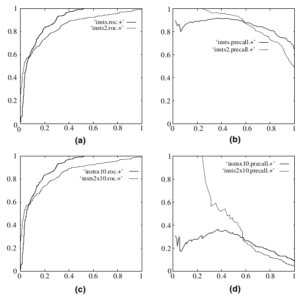
ROC 曲线的特点

当测试集中的 正负样本的分布变化 的时候，ROC曲线能够保持不变
(a)(c) 为 ROC 曲线，(b)(d) 为 Precision-Recall 曲线
- $Precision={ {\color{red}TP} \over {\color{red}TP} + {\color{green}FP} }$
- $Recall=TPR={ {\color{red}TP} \over {\color{red}TP} + {\color{red}FN} }$
(c)(d) 将测试集中 负样本的数量增加到原来的 10 倍，ROC 曲线较为稳定，而 PR 曲线变化很大
在实际的数据集中经常会出现 类不平衡现象，即负样本比正样本多很多 (或者相反)，而且测试数据中的正负样本的分布也可能随着时间变化。在这种情况下，ROC 曲线在评估上有 更好的稳定性
PR 曲线在正负样本分布得极不均匀时，能更有效地反映模型的好坏

图片来源：https://www.plob.org/article/12476.html

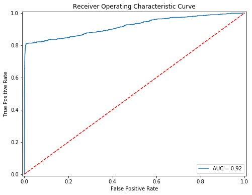
7.2 利用 AUC 评估逻辑回归模型准确性

import matplotlib.pyplot as plt
from sklearn.metrics import roc_auc_score
from sklearn.model_selection import train_test_split
from sklearn.externals import joblib
import pandas as pd
from sklearn import metrics
data = pd.read_table('dataset13.txt',sep='\t')
y = data['Default'].values
x = data.drop(['Default'], axis=1).values
# 划分训练集和测试集
x_train, x_test, y_train, y_test = train_test_split(
  x, y, test_size=0.2,random_state = 33,stratify=y)
# 加载模型
lr = joblib.load("train_model.m")
y_predict = lr.predict_proba(x_test)[:,1]

#用metrics.roc_curve()求出 fpr, tpr, threshold
fpr, tpr, threshold = metrics.roc_curve(
  y_test, y_predict)
#用metrics.auc求出roc_auc的值
roc_auc = metrics.auc(fpr, tpr)
import matplotlib.pyplot as plt
from sklearn.metrics import roc_auc_score
from sklearn.model_selection import train_test_split
from sklearn.externals import joblib
import pandas as pd
from sklearn import metrics
data = pd.read_table('dataset13.txt',sep='\t')
y = data['Default'].values
x = data.drop(['Default'], axis=1).values
# 划分训练集和测试集
x_train, x_test, y_train, y_test = train_test_split(
  x, y, test_size=0.2,random_state = 33,stratify=y)
# 加载模型
lr = joblib.load("train_model.m")
y_predict = lr.predict_proba(x_test)[:,1]

#用metrics.roc_curve()求出 fpr, tpr, threshold
fpr, tpr, threshold = metrics.roc_curve(
  y_test, y_predict)
#用metrics.auc求出roc_auc的值
roc_auc = metrics.auc(fpr, tpr)

#将图片大小设为8:6
fig,ax = plt.subplots(figsize=(8,6))

#将plt.plot里的内容填写完整
plt.plot(fpr, tpr, label = f'AUC = {roc_auc:.2f}')
 
#将图例显示在右下方
plt.legend(loc = 'lower right') 
 
#画出一条红色对角虚线
plt.plot([0, 1], [0, 1],'r--') 
 
#设置横纵坐标轴范围
plt.xlim([-0.01, 1.01]) 
plt.ylim([-0.01, 1.01])
 
#设置横纵名称以及图形名称
plt.ylabel('True Positive Rate')
plt.xlabel('False Positive Rate')
plt.title('Receiver Operating Characteristic Curve')
plt.show()
#将图片大小设为8:6
fig,ax = plt.subplots(figsize=(8,6))

#将plt.plot里的内容填写完整
plt.plot(fpr, tpr, label = f'AUC = {roc_auc:.2f}')
 
#将图例显示在右下方
plt.legend(loc = 'lower right') 
 
#画出一条红色对角虚线
plt.plot([0, 1], [0, 1],'r--') 
 
#设置横纵坐标轴范围
plt.xlim([-0.01, 1.01]) 
plt.ylim([-0.01, 1.01])
 
#设置横纵名称以及图形名称
plt.ylabel('True Positive Rate')
plt.xlabel('False Positive Rate')
plt.title('Receiver Operating Characteristic Curve')
plt.show()

7.2 利用 AUC 评估逻辑回归模型准确性

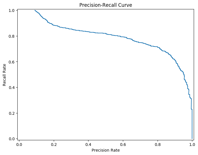
使用 PR 曲线呈现

pre, rec, the2 = metrics.precision_recall_curve(
  y_test, y_predict
)
plt.plot(pre, rec)

plt.xlim([-0.01, 1.01]) 
plt.ylim([-0.01, 1.01])

plt.ylabel('Recall Rate')
plt.xlabel('Precision Rate')
plt.title('Precision-Recall Curve')
plt.show()
pre, rec, the2 = metrics.precision_recall_curve(
  y_test, y_predict
)
plt.plot(pre, rec)

plt.xlim([-0.01, 1.01]) 
plt.ylim([-0.01, 1.01])

plt.ylabel('Recall Rate')
plt.xlabel('Precision Rate')
plt.title('Precision-Recall Curve')
plt.show()

因为本实验中，正负样本分布不均匀，因此 PR 曲线呈现出的效果也有一定的参考价值

7.3 利用 AUC 评估随机森林模型准确性

from sklearn.metrics import roc_auc_score
from sklearn.model_selection import train_test_split
import pandas as pd
from sklearn.externals import joblib
from sklearn import metrics
import matplotlib.pyplot as plt
data = pd.read_table('dataset13.txt',sep='\t')
y = data['Default'].values
x = data.drop(['Default'], axis=1).values
# 划分训练集和测试集
x_train, x_test, y_train, y_test = train_test_split(
  x, y, test_size=0.2,random_state = 33,stratify=y)
# 加载模型
rf_clf = joblib.load("train_model2.m")
y_predict = rf_clf.predict_proba(x_test)[:,1]
#用metrics.roc_curve()求出 fpr, tpr, threshold
fpr, tpr, threshold = metrics.roc_curve(
  y_test, y_predict)

#用metrics.auc求出roc_auc的值
roc_auc = metrics.auc(fpr, tpr)
from sklearn.metrics import roc_auc_score
from sklearn.model_selection import train_test_split
import pandas as pd
from sklearn.externals import joblib
from sklearn import metrics
import matplotlib.pyplot as plt
data = pd.read_table('dataset13.txt',sep='\t')
y = data['Default'].values
x = data.drop(['Default'], axis=1).values
# 划分训练集和测试集
x_train, x_test, y_train, y_test = train_test_split(
  x, y, test_size=0.2,random_state = 33,stratify=y)
# 加载模型
rf_clf = joblib.load("train_model2.m")
y_predict = rf_clf.predict_proba(x_test)[:,1]
#用metrics.roc_curve()求出 fpr, tpr, threshold
fpr, tpr, threshold = metrics.roc_curve(
  y_test, y_predict)

#用metrics.auc求出roc_auc的值
roc_auc = metrics.auc(fpr, tpr)

#将图片大小设为8:6
fig,ax = plt.subplots(figsize=(8,6))

#将plt.plot里的内容填写完整
plt.plot(fpr, tpr, label = f'AUC = {roc_auc:.2f}')

#将图例显示在右下方
plt.legend(loc = 'lower right') 

#画出一条红色对角虚线
plt.plot([0, 1], [0, 1],'r--') 

#设置横纵坐标轴范围
plt.xlim([-0.01, 1.01]) 
plt.ylim([-0.01, 1.01])

#设置横纵名称以及图形名称
plt.ylabel('True Positive Rate')
plt.xlabel('False Positive Rate')
plt.title('Receiver Operating Characteristic Curve')
plt.show()
#将图片大小设为8:6
fig,ax = plt.subplots(figsize=(8,6))

#将plt.plot里的内容填写完整
plt.plot(fpr, tpr, label = f'AUC = {roc_auc:.2f}')

#将图例显示在右下方
plt.legend(loc = 'lower right') 

#画出一条红色对角虚线
plt.plot([0, 1], [0, 1],'r--') 

#设置横纵坐标轴范围
plt.xlim([-0.01, 1.01]) 
plt.ylim([-0.01, 1.01])

#设置横纵名称以及图形名称
plt.ylabel('True Positive Rate')
plt.xlabel('False Positive Rate')
plt.title('Receiver Operating Characteristic Curve')
plt.show()

模型报错了！

6.12 使用网格搜索进行随机森林参数调优

import ...
data = pd.read_table('dataset13.txt',sep='\t')
y = data['Default'].values
x = data.drop(['Default'], axis=1).values
x_train, x_test, y_train, y_test = train_test_split(x, y, test_size=0.2,random_state = 33,stratify=y)

rf = RandomForestClassifier()

# 设置需要调试的参数
tuned_parameters = {'n_estimators': [180,190],'max_depth': [8,10]}

# 调用网格搜索函数
rf_clf = GridSearchCV(rf, tuned_parameters, scoring='roc_auc', n_jobs=2, cv=5)
rf_clf.fit(x_train, y_train)

y_predict = rf_clf.predict_proba(x_test)[:, 1]
test_auc = roc_auc_score(y_test, y_predict)
print ('随机森林模型test AUC:')
print (test_auc)
joblib.dump(rf_clf, 'train_model2.m')
import ...
data = pd.read_table('dataset13.txt',sep='\t')
y = data['Default'].values
x = data.drop(['Default'], axis=1).values
x_train, x_test, y_train, y_test = train_test_split(x, y, test_size=0.2,random_state = 33,stratify=y)

rf = RandomForestClassifier()

# 设置需要调试的参数
tuned_parameters = {'n_estimators': [180,190],'max_depth': [8,10]}

# 调用网格搜索函数
rf_clf = GridSearchCV(rf, tuned_parameters, scoring='roc_auc', n_jobs=2, cv=5)
rf_clf.fit(x_train, y_train)

y_predict = rf_clf.predict_proba(x_test)[:, 1]
test_auc = roc_auc_score(y_test, y_predict)
print ('随机森林模型test AUC:')
print (test_auc)
joblib.dump(rf_clf, 'train_model2.m')

将训练好的模型下载后，上传至 7.3

7.3 利用 AUC 评估随机森林模型准确性

工具：Slidev
绘图：p5.js